DMFTLab Library
Documentation
Table of Content
3. Computing Properties: Overview
A.1 Computing Spectral Functions at Imaginary Axis
A.2 Computing Spectral Functions at Real Axis
B.1 Visualizing Spectral Functions at Imaginary Axis
B.2 Visualizing Spectral Functions at Real Axis
C.1 Accessing General Properties
C.2 Accessing Interactions Properties
D.1 Setting General Properties for a Level
E.1 Accessing Method Convergency Options
E.2 Accessing Method Mixings Options
© Copyright 2005 University
of California Davis
1. Ove rview
of DMFTLab
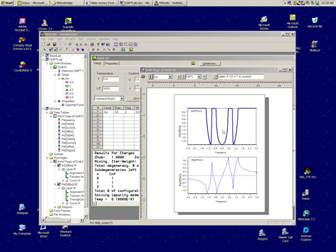
Welcome to DMFTLab, the scientific software for Windows systems that
performs calculations of properties of several most popular versions of model
hamiltonians. DMFTLab is a library dynamically linked to MStudio. DMFTLab also
uses MScene library for visualization.
DMFTLab consists of a window that is used to set up input data, perform
calculations and analyze output data. The DMFTLab Window, shortly DMFT Window
is called using DmftLab command of the Project menu or
corresponding button of the DMFTLab Toolbar.
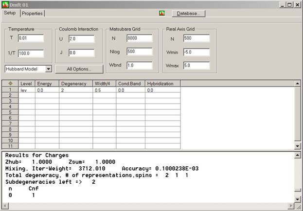
The DMFT window consists of two Property Pages:
- Setup Page
- Properties Page
 A lower area of the DMFT Window is an output
area where the output of the calculation is shown.
A lower area of the DMFT Window is an output
area where the output of the calculation is shown.
The engine of the DMFTLab is a program called LmtART. The LmtART is
an executable file that reads the input data, performs calculation, and stores
the output files. The DMFT Window only controls this process, it prepares input
for the LmtART using dialog windows, and starts LmtART program as a separate
thread. When the calculation is finished, LmtART notifies the DMFTLab, and the
output files are read by the DMFT Window and can be visualized by simple mouse
click operations.
While running LmtART program for complicated setups can be rather slow,
the DMFTLab can be used to prepare the input files, after which they can be
copied to another computer where the LmtART can be run in a faster way. After
run is performed, the output files can be copied back to the PC and DMFTLab can
analyze them quickly. All input/output files are formatted, and therefore
system independent.
The DMFTLab uses scratch directory to run LmtART program. By default
scratch directory is called LmtRUN. It exists at the MStudio installation
directory. All input/output files prepared by the DMFT window are stored in
this directory.
A separate issue of the DMFTLab is its Database. The DMFTLab has a
database of various setups that have been calculated using the LmtART program.
The database is an important part of the library, it can be called by pressing DataBase
button located on the top right part of the DMFT Window. The input/output
files can be stored within the database: this gives possibility to use these
files on the remote machines. Refer to Using DataBase topic for
the detailed discussion.
2. Setting DMFT Data: Ove rview
The first property page of the DMFT Window is designed to describe model hamiltonian parameters:
- Temperature or reciprocal temperature
- Model hamiltonian choice
- Intraatomic Coulomb interaction parameters
U and J
- Imaginary axis grid settings
- Real axis grid setting
More options can be
accessed via clicking Access All Options button. The corresponding
property pages are
- General Properties
- Interactions Properties
- Grids Properties
The following set of
data has to be given for each impurity level
- Level title, like “s-level”, “p-level”. If
spin polarization is desired, specify in the title either “-up”, or “-dn”
ke
- Energy of the impurity level. Note that
the energy has to be set with respect to particle hole-symmetry point,
i.e. it is doping position. If bare position of impurity level is Ef, the
doping position is Ef-U(N-1)/2, where U is Hubbard U parameter set up
above.
- Degeneracy of the level.
- Quarter of bandwidth. For the Hubbard
model this is quarter of bandwidth of the band. For the periodic
- Conduction band position. This option is
only necessary for the periodic
- Hybridization between the conduction band
and impurity level. This option is only necessary for the periodic
Additional options for atoms can be accessed by highlighting the entire
row and calling the Properties dialog box with the right mouse button.
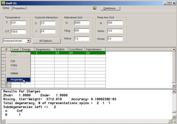
Another possibility to call the Level Properties dialog box is to access
it from the Object Explorer.
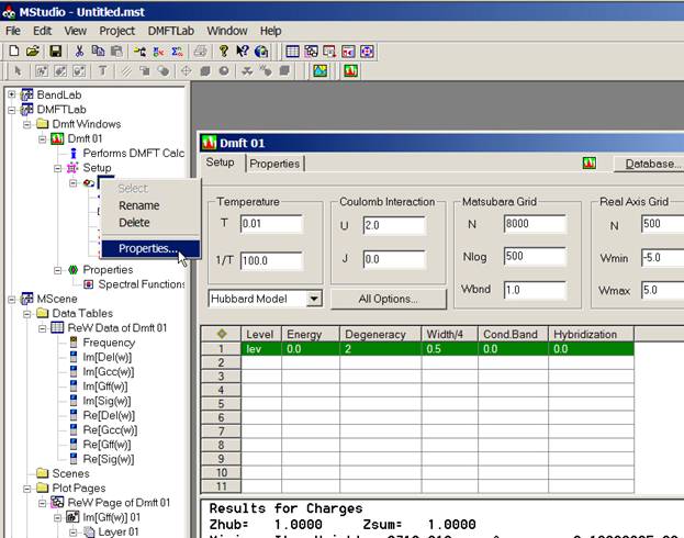
The dialog box which allows to access various properties for the selected level appears. These properties include:
- General Properties
3. Computing Properties: Ove rview
Computation of properties of model hamiltonians is the goal of the DMFTLab
library. The LmtART
program is the executable module that does this calculation. It reads input
files prepared by the DMFT Window, performs the calculation of the desired
property, and notifies the DMFT Window again that the calculation is finished.
The DMFTLab reads the output files and visualizes them with help of the MScene
library.
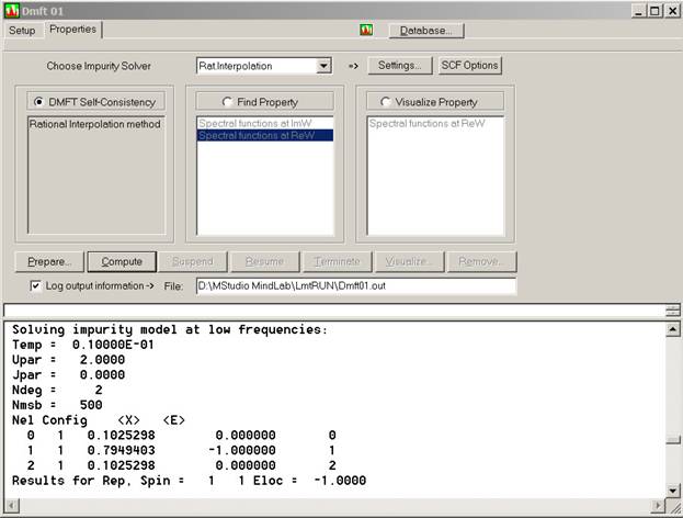
The purpose of the Properties page of the DMFT Window is to make final
preparations before starting LmtART, start LmtART code, and visualize the
output data computed by the LmtART. Once the data are set using Setup property page,
the last step is to choose the method of computing the physical property.
Several methods are
currently available within the use of DMFTLab library:
- Hubbard I method
- Slave-boson mean field method.
- Rational Interpolation method
Each method has its own set of options which can be set by clicking Settings.
A set of options to perform self-consistency can be accessed via clicking SCF
Options button. It includes
- Convergence
criteria
- Mixing options
All methods perform DMFT self-consistent calculation to find spectral
functions at imaginary axis. To make self-consistency, switch on radio button Make
Self-Consistency and click Compute button. The self-consistent
calculation will start. The output window in the lower part of the DMFT Window
will show haw the self-consistent process is performed. This however maybe
rather slow process. At the end of the calculation, the framework creates the
file consisting the self-consisting spectral functions data.
Once self-consistency is performed, physical properties can be computed.
To compute physical property such as Spectral Functions in Real Axis,
set radio button Find Property to the On position. Chose the property from the drop-down list
and press Compute button. ( You may also use Prepare button to
set more options before pressing compute button.)
The following set of
properties can be computed by the DMFTLab:
- Spectral Functions at Imaginary Axis
- Spectral Functions at Real Axis
After the computation of a particular property is finished, the
framework will add this into the computed properties list of the Visualize
Property drop-down list.
To start visualizing the properties that have been computed, choose
radio button Visualize Property. Highlight corresponding property and
press Visualize button. A visualization dialog box appears. You can
start visualizing the data by pressing Visualize with the current settings
button in the lower part of this dialog box.
The following controls
help to visualize the computed properties:
- Visualzing Spectral Functions at Imaginary
Axis
- Visualizing Spectral Functions at Real
Axis
All visualization
plots can be additionally customized using the commands of MScene library.
Refer to the MScene Library documentation for corresponding instructions.
4. Using DMFT DataBase: Ove rview
The integrated database is important part of the DMFTLab library. Instead of maintaining its own input files, one can use database to extract set-ups for similar problems and then slightly modify them. After computation of the properties and or self-consistency process is performed one can store the computed data into the database to be able to use them in the future runs.
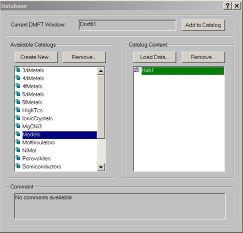
To call database press Database button located at the top right
part of the DMFT window. The database dialog box appears. The database consists
of catalogs and their contents. A set of predefined catalogs describing set-ups
for some simple models is provided with this installation.
To load data from the database into the DMFT Window select a particular model
and press Load Data button. To store data computed by the DMFT Window,
use button Add to Catalog located on the top of the database dialog box.
New catalogs can be created and removed. Entries within the catalog can
also be removed using corresponding buttons.
In fact, the database maintained by the framework is located in the
database folder of the directory where installation of MStudio has been
performed. Navigate database folder, the input and output files for many
different examples are stored in its subdirectories. All these files are either
input or output files of the LmtART program that performs actual computations.
Refer to the LmtART manual for detailed instructions about input and output to
this program.
5. LmtART program
LmtART is free scientific software designed to perform electronic structure calculations of the materials. It is written using Fortran 90 programming language and uses full dynamical memory model. The source codes for that program, as well as installation and operating instructions can be downloaded from the same site as the MStudio, MScene, BandLab, and DMFTLab libraries. Refer to specific license agreement and copyright notice when using LmtART codes.
A.1 Computing Spectral Functions at Imaginary Axis
To compute density spectral functions at imaginary axis, the self-consistent DMFT loop is used. The paramters of self-consistent cycle can be chosen.
A.2 Computing Spectral Functions at Real Axis
To compute density spectral functions at real axis, the self-consistent DMFT loop is used. The parameters of self-consistent cycle can be chosen.
B.1 Visualizing Spectral Functions at Imaginary Axis
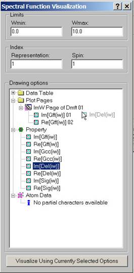 In
order to visualize spectral functions, use Visualize Spectral Functions
dialog box. Enter lower and upper frequency limits. For crystal filed case or
spin polarized case you may setup which representation and spin to visualize.
If representation and/or spin is set to zero, a sum over all representations
and/or spins will be performed. This makes sense for such properties as the
Density of States only.
In
order to visualize spectral functions, use Visualize Spectral Functions
dialog box. Enter lower and upper frequency limits. For crystal filed case or
spin polarized case you may setup which representation and spin to visualize.
If representation and/or spin is set to zero, a sum over all representations
and/or spins will be performed. This makes sense for such properties as the
Density of States only.
A special tree control exists to set up which spectral functions should be drawn. Drag them from the Property folder and drop them within the Page folder into the icon showing the Page. Note that you can use right mouse button to access to the pop-up menu with Rename, Delete, Add commands. You can add new Pages and drag calculated properties to every of these pages. In this way, you can set up spontaneously several pages with each page containing several graphs. When you are done with the descriptions of graphs, press Visualize button at the button. The program will use the graphical library to draw selected set of properties.
B.2 Visualizing Spectral Functions at Real Axis
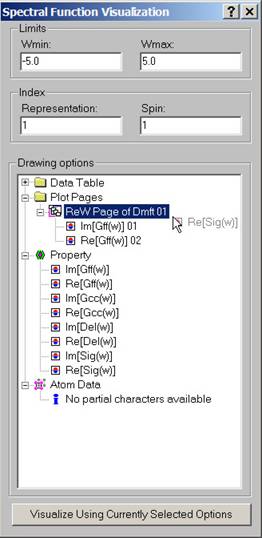 In
order to visualize spectral functions, use Visualize Spectral Functions
dialog box. Enter lower and upper frequency limits. For crystal filed case or
spin polarized case you may setup which representation and spin to visualize.
If representation and/or spin is set to zero, a sum over all representations
and/or spins will be performed. This makes sense for such properties as the
Density of States only.
In
order to visualize spectral functions, use Visualize Spectral Functions
dialog box. Enter lower and upper frequency limits. For crystal filed case or
spin polarized case you may setup which representation and spin to visualize.
If representation and/or spin is set to zero, a sum over all representations
and/or spins will be performed. This makes sense for such properties as the
Density of States only.
A special tree control exists to set up which spectral functions should be drawn. Drag them from the Property folder and drop them within the Page folder into the icon showing the Page. Note that you can use right mouse button to access to the pop-up menu with Rename, Delete, Add commands. You can add new Pages and drag calculated properties to every of these pages. In this way, you can set up spontaneously several pages with each page containing several graphs. When you are done with the descriptions of graphs, press Visualize button at the button. The program will use the graphical library to draw selected set of properties.
C.1 Accessing General Properties
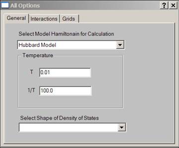 Describe
general properties such as model hamiltonian choice, temperature and the shape
of non-interacting density of states.
Describe
general properties such as model hamiltonian choice, temperature and the shape
of non-interacting density of states.
C.2 Accessing Interactions Properties
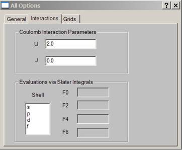 Intraatomic Coulomb
interaction parameters, Hibbard U and exchange J are set using this property
page.
Intraatomic Coulomb
interaction parameters, Hibbard U and exchange J are set using this property
page.
Their evaluations can be done using Slater integrals by selecting the corresponding l shell of the atom.
C.3 Accessing Grids
 Imaginary
axis (Matsubara grid) settings are described by a number of points and the
temperature. Logarithmic grid is used to accelerate the calculation. It is set
by the number of points and the effective bandwidth. The cutoff frequency will
be evaluated automatically from these settings
Imaginary
axis (Matsubara grid) settings are described by a number of points and the
temperature. Logarithmic grid is used to accelerate the calculation. It is set
by the number of points and the effective bandwidth. The cutoff frequency will
be evaluated automatically from these settings
To compute the spectral functions at real axis, specify minimal and maximal frequency as well as the number of points.
D.1 Setting Properties for a Level
 Description of the
correlated level.
Description of the
correlated level.
- Level title, like “s-level”, “p-level”. If
spin polarization is desired, specify in the title either “-up”, or “-dn”
ke
- Energy of the impurity level. Note that
the energy has to be set with respect to particle hole-symmetry point,
i.e. it is doping position. If bare position of impurity level is Ef, the
doping position is Ef-U(N-1)/2, where U is Hubbard U parameter set up
above.
- Degeneracy of the level.
- Quarter of bandwidth. For the Hubbard
model this is quarter of bandwidth of the band. For the periodic
- Conduction band position. This option is
only necessary for the periodic
- Hybridization between the conduction band
and impurity level. This option is only necessary for
the periodic
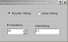
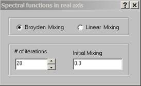
E.1 Accessing Method Convergency Options
 Settings
for DMFT self-consistency loops both at imaginary and real axis can be
specified as well as convergency criterium.
Settings
for DMFT self-consistency loops both at imaginary and real axis can be
specified as well as convergency criterium.
E.2 Accessing Method Mixings Options
 Mixing
options for both Broyden and linear mixing schemes can be specified including
the choice of mixing function.
Mixing
options for both Broyden and linear mixing schemes can be specified including
the choice of mixing function.
F.1 Accessing Method Settings
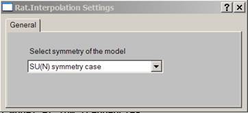 Each method has its own set of additional options. For
fully degenerate model select SU(N) symetry case. For levels split by crystal
fields, select crystal field splitted case.
Each method has its own set of additional options. For
fully degenerate model select SU(N) symetry case. For levels split by crystal
fields, select crystal field splitted case.